How to create a Venn Diagram in R

news

code

analysis

Short guide on how to create a Venn Diagram with code provided

Author

Jakob Johannesson

Published

October 24, 2022

Simple Venn Diagram (Two circles)

Code

# Venn diagram with ggplot

library(tidyverse)
library(ggforce)    # Adds geom_circle

# DataFrame to specify circle and text positions
data <- data.frame(x = c(1, -1),
                   y = c( 1, 1),
                   tx = c(1.5, -1.5),
                   ty = c(1.3, 1.3),
                   cat = c("Studenter", 
                           "Nykterister"))



# Plot circles and text; add annotations for overlapping segments
ggplot(data, aes(x0 = x , y0 = y, r = 1.5, fill = cat)) + 
  geom_circle(alpha = 0.25, size = 1, color = "black",show.legend = FALSE) + 
  geom_text(aes(x = tx , y = ty, label = cat), size = 12) +
  annotate(geom="text", x=0, y=1.2, label="Nyktra\nStudenter",color="red3", size = 14) +
  #annotate(geom="text", x=-1.5, y=0.7, label="Antal i Sverige: 4 871 000",color="darkgreen", size = 11.5) +
  #annotate(geom="text", x=1.5, y=0.7, label="Antal i Sverige: 712 000",color="darkgreen", size = 11.5) +
  #annotate(geom="text", x=0, y=0.8, label="Antal: ?",color="darkgreen", size = 16) +
  theme_void()

Adding labels to Venn Diagram

Code

data <- data.frame(x = c(1, -1),
                   y = c( 1, 1),
                   tx = c(1.5, -1.5),
                   ty = c(1.3, 1.3),
                   cat = c("Studenter", 
                           "Nykterister"))

ggplot(data, aes(x0 = x , y0 = y, r = 1.5, fill = cat)) + 
  geom_circle(alpha = 0.25, size = 1, color = "black",show.legend = FALSE) + 
  geom_text(aes(x = tx , y = ty, label = cat), size = 12) +
  annotate(geom="text", x=0, y=1.3, label="Nyktra\nStudenter",color="red3", size = 14) +
  annotate(geom="text", x=-1.5, y=0.7, label="Antal i Sverige: 71k",color="darkgreen", size = 11.5) +
  annotate(geom="text", x=1.5, y=0.7, label="Antal i Sverige: 1.2k",color="darkgreen", size = 11.5) +
  annotate(geom="text", x=0, y=0.65, label="Antal:\n?",color="darkgreen", size = 11) +
  theme_void()

Three circles

Code

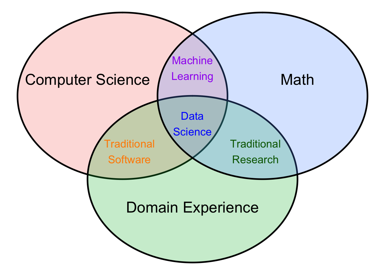
# DataFrame to specify circle and text positions
data <- data.frame(x = c(0, 1, -1),
                   y = c(-0.5, 1, 1),
                   tx = c(0, 1.5, -1.5),
                   ty = c(-1, 1.3, 1.3),
                   cat = c("Domain Experience", "Math", 
                           "Computer Science"))


ggplot(data, aes(x0 = x , y0 = y, r = 1.5, fill = cat)) + 
  geom_circle(alpha = 0.25, size = 1, color = "black",show.legend = FALSE) + 
  geom_text(aes(x = tx , y = ty, label = cat), size = 7)+
  annotate(geom="text", x=0, y=1.5, label="Machine\nLearning",color="purple", size = 5) +
  annotate(geom="text", x=-0.9, y=0, label="Traditional\nSoftware",color="darkorange", size = 5) +
  annotate(geom="text", x=0.9, y=0, label="Traditional\nResearch",color="darkgreen", size = 5) +
  annotate(geom="text", x=0, y=0.5, label="Data\nScience",color="blue", size = 5) +
  theme_void()

Four circles (Ikigai)

Code

data <- data.frame(x = c(1, 0, -1, 0),
                   y = c(0, 1, 0, -1),
                   tx = c(1.8, 0, -1.8, 0),
                   ty = c(0, 1.8, 0, -1.8),
                   cat = c("Needs", "Love", 
                           "Good at","Paid for"))


ggplot(data, aes(x0 = x , y0 = y, r = 1.5, fill = cat)) + 
  geom_circle(alpha = 0.25, size = 1, color = "black",show.legend = FALSE) + 
  geom_text(aes(x = tx , y = ty, label = stringr::str_to_upper(cat)), size = 7) +
  annotate(geom="text", x=0, y=0.0, label="Ikigai",color="red3", size = 8) +
  theme_void()

Enjoy this small introduction to Venn Diagrams in R!